Appendix D: Kalman filtering

The system of considering the Kalman filtering problem is a linear stochastic state-observation description as follows:

$${{\bf {x}}}_{m+1}={\bf {F}}_m {\bf {x}}_m + {\bf {G}}_m {\bf {w}}_m \mbox{({\bf {state}})}$$

$${{\bf {y}}_m}={\bf {H}}_m {\bf {x}}_m + {\bf {v}}_m \mbox{({\bf {observation}})},$$

where ${\bf {x}}_m$ and ${\bf {y}}_m$ are random variables, and ${\bf {F}}_m$, ${\bf {G}}_m$, and ${\bf {H}}_m$, are state transition matrix, observation matrix, and driving matrix, respectively.

In this system, mean and variance with ${\rm {x}}_0$, ${\rm {w}}_m$, and ${\rm {v}}_m$ are known. And ${\bf {F}}_m$, ${\bf {G}}_m$, ${\bf {H}}_m$, and ${\bf {v}}_m$ are known matrices. The Kalman filtering problem is to determine the minimum variance requirement $\hat{\rm {x}}_{m\vert m}$ from the observed ${\rm {y}}_m$, $m=0,1,2, \cdots, M$ as follows.

$$\hat{\rm {x}}_{m\vert m}=E({\rm {x}}_m+{\bf {y}}_0,\cdots, {\rm {y}}_m)$$ (56)

The Kalman filter is called an algorithm that obtains a solution to the above problem [Brown and Hwang1992].

It is calculated by sequentially performing the following:[Brown and Hwang1992].

1.

Filtering equation

$$\hat{{\bf {x}}}_{m\vert m}=\hat{{\bf {x}}}_{m\vert m-1}+{\bf {K}}_m({\bf {y}}_m-{\bf {H}}_m\hat{{\bf {x}}}_{m\vert m-1})$$ (57)

$$\hat{{\bf {x}}}_{m+1\vert m}={\bf {F}}_m\hat{{\bf {x}}}_{m\vert m}$$ (58)

2.

Kalman gain

$${\bf {K}}_m=\frac{\hat{{\bf {\Sigma}}}_{m\vert m-1}{\bf {H}}_... ... {\Sigma}}}_{m\vert m-1}{\bf {H}}_m^{*T}+{\bf {\Sigma}}_{v_m}}$$ (59)

3.

Covariance equation for the estimated-error

$$\hat{{\bf {\Sigma}}}_{m\vert m}=\hat{\bf {\Sigma}}_{m\vert m-1}-{\bf {K}}_m {\bf {H}}_m \hat{{\bf {\Sigma}}}_{m\vert m-1}$$ (60)

$$\hat{{\bf {\Sigma}}}_{m+1\vert m}=\hat{\bf {F}}_m{\bf {\Sigma}}_{m\vert m}{\bf {F}}_m^{*T}+{\bf {G}}_m {\bf {\Sigma}}_{w_m}{\bf {G}}_m^{*T}$$ (61)

4.

Initial state

$$\hat{\bf {x}}_{0\vert-1}=\bar{\bf {x}}_0, \qquad \hat{\bf {\Sigma}}_{0\vert-1}={\bf {\Sigma}}_{x_0},$$ (62)

We remark that symbols $\bar{\qquad}$ and ${\bf {\Sigma}}$ are mean and variance of a random variable, respectively.

  

Figure 1: Auditory segregation model.

  

Figure 2: Vector-plane of complex spectrum.

  

Figure 3: Overview of signal-flow in the proposed model.

  

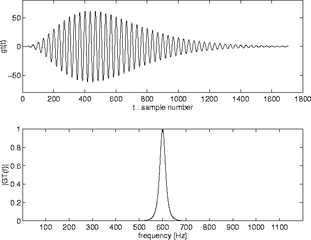
Figure: Characteristics of basic wavelet $\psi (t)$: (top panel) ${\rm {Re}}\{\psi (t)\}$, (bottom panel) $\hat{\psi}(f)$(gammatone filter at f₀=600 Hz, N=4, b_f=0.25).

  

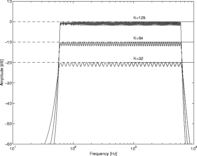
Figure 5: Frequency characteristics of the wavelet filterbank (the criterion levels are 0 dB for K=128; -10 dB for K=64; and -20 dB for K=32.).

  

Figure 6: Temporal variation of the fundamental frequency.

  

Figure 7: Candidates for C_k(t) interpolated by the spline function.

      

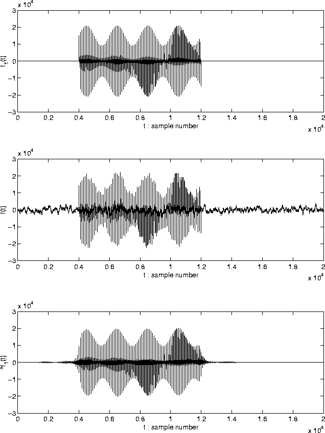
Figure 8: AM complex tone f₁(t).
Figure 9: Mixed signals f(t) (SNR=10 dB).
Figure: Extracted signal $\hat{f}_1(t)$.

  

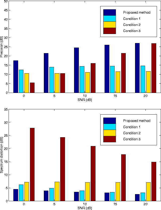
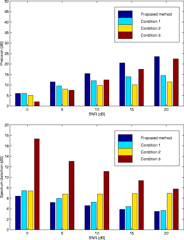
Figure: Segregation accuracy for simulation 1: (top panel) precision for the A_k(t), (bottom panel) spectrum distortion for the extracted signal $\hat{f}_1(t)$.

    

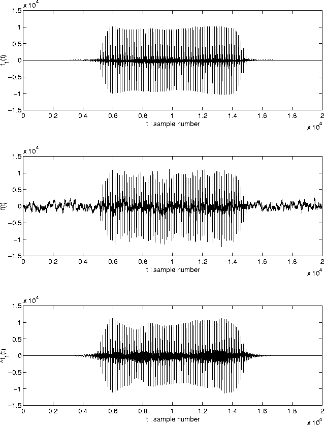
Figure 12: Mixed signals f(t) (SNR=10 dB).
Figure: Extracted signal $\hat{f}_1(t)$.

  

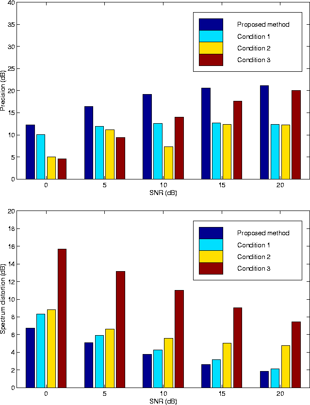
Figure: Segregation accuracy for simulation 2: (top panel) precision for the A_k(t), (bottom panel) spectrum distortion for the extracted signal $\hat{f}_1(t)$.

      

Figure 15: LMA-synthesized vowel /a/ f₁(t).
Figure 16: Mixed speech f(t) (SNR=10 dB).
Figure: Extracted vowel /a/ $\hat{f}_1(t)$.

  

Figure: Segregation accuracy for simulation 3: (top panel) precision for the A_k(t), (bottom panel) spectrum distortion for the extracted signal $\hat{f}_1(t)$.

  

Figure: Comparison of the amplitude spectrum of $\hat{f}_1(t)$ with the amplitude spectrum of f₁(t).

 

Table I: Definitions of symbols for the segregation problem.

Symbol	Definition
Sk(t)	instantaneous amplitude
$\phi _k(t)$	instantaneous output phase
Ak(t), Bk(t)	instantaneous amplitude
$\theta_{1k}(t),\theta_{2k}(t)$	instantaneous input phases
$\theta_k(t)$	input phase difference
F0(t)	Fundamental frequency
Ck,R(t), Dk,R(t),	R-th-order polynomial
$\quad E_{0,R}(t)$	$\qquad$(differentiable, piecewise)
Ck(t)	undetermined function

 

 

Table II: Constraints corresponding to Bregman's regularities.

Heuristic regularity (Bregman, 1993)	Constraint
(i) Unrelated sounds seldom start or stop at exactly	Synchronous of onset and offset
the same time.
(ii) Gradualness of change.	Gradualness of change
(a) A single sound tends to change its properties	(piecewise-differentiable polynomial
smoothly and slowly.	approximation and smoothness)
(b) A sequence of sounds from the same source	(piecewise-differentiable polynomial
tends to change its properties slowly.	approximation and smoothness)
(iii) When a body vibrates with a repetitive period,	Harmonicity
this vibrations give rise to an acoustic pattern
in which the frequency components are
multiples of a common fundamental.
(iv) Many changes that take place in an acoustic	Correlation between the
event will affect all the components of the	instantaneous amplitudes
resulting sound in the same way and at
the same time.

 

 

Table III: Specifications of the filterbank design

Symbol	Definition
fs	sampling frequency	20 kHz
K	channel number	128
W	bandwidth	60 Hz - 6 kHz
a	scale parameter	$\alpha^p$
$\alpha$	scale	102/K
p	index	$-\frac{K}{2} \leq p \leq \frac{K}{2}$
b	dilation	q/fs
q	index	$q\in {\bf {Z}}$

 

 

Table IV: Definitions of symbol for the Kalman filter.

Symbol	Definition
observed signal	${\bf {y}}_m=X_k(t_m)$
state variable	${\bf {x}}_m=-C_{k,0}(t_m)$
observed noise	${\bf {v}}_m=X_{2,k}(t_m)$
system noise	${\bf {w}}_m=w_m$
state transition matrix	${\bf {F}}_m=\Delta C_k(t_m)$
observation matrix	${\bf {H}}_m=e^{j\omega_k t_m}$
driving matrix	${\bf {G}}_m=-1$