Evaluation measures

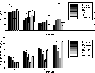
We used two measures to evaluate the segregation performance of the proposed method.

One was the ratio of the original f₁(t) (signal) and the difference between the original and the segregated signal $\hat{f}_1(t)$ (noise), as defined by

$$10\log_{10}\frac{\int_0^T f_1(t)^2dt}{\int_0^T (f_1(t)-\hat{f}_1(t))^2dt}. \qquad {\rm {(dB)}}$$ (16)

The aim of using this measure was to evaluate whether a segregation model can segregate a desired signal from a noisy signal precisely even in waveforms. This measure is called ``segregation accuracy.''

The other measure was an objective distortion estimator for hearing aids such as the spectrum distortion reconsidered with the simultaneous and temporal masking effects. This measure is defined by

$$\sqrt{\frac{1}{W}\sum_\omega^W \left(20\log_{10} \frac{\tilde... ...ga)}{\tilde{\hat{X}}_1(\omega)}\right)^2}, \qquad {\rm {(dB)}}$$ (17)

where $\tilde{X}_1(\omega)$ and $\tilde{\hat{X}}_1(\omega)$ are the amplitude spectra of f₁(t) and $\hat{f}_1(t)$, respectively. This is called ``auditory-oriented spectral distortion (ASD)'' [Mizumachi and Akagi1999]. In the above equation, the frame length is 21.3 ms, the frame shift is a quarter of the frame length, W is the analyzable bandwidth of the filterbank (about 6 kHz), the sampling frequency is 48 kHz, and the window function is Hamming [Mizumachi and Akagi1999]. Since the sampling frequency of our model is 20 kHz, we have to do an up-sampling of 20 kHz to 48 kHz to use the ASD.

    

Figure: ASD for simulation 1: (a) bandpassed pink noise, (b) bandpassed white noise.
Figure: Segregation accuracy for simulation 1: (a) bandpassed pink noise, (b) bandpassed white noise.

    

Figure: ASD for simulation 2: (a) bandpassed pink noise, (b) bandpassed white noise.
Figure: Segregation accuracy for simulation 2: (a) bandpassed pink noise, (b) bandpassed white noise.

    

Figure: ASD for simulation 3.
Figure: Segregation accuracies for simulation 3.